Question 1
Students seeking support with similar academic tasks can explore best assignment help Australia for assistance across a range of subjects.
1a: Decision Variables
In this problem, three decision variables are used. These are the number of units produced for Product1, Product2, and Product3. Each variable represents the production quantity that the company can decide on. The purpose of identifying these variables is to allow Solver to change their values and find the best combination. By focusing on these three decisions, the business can check how different production levels affect total profit while staying within resource limits.
1b: Nature of the Problem
This optimization problem is a maximisation problem. The aim is to earn as much profit as possible from the three products. Since profit increases when more products are made, subject to resource restrictions, Solver is set to maximise the total profit value (Cohen, Lee & Song, 2021). It is not a minimisation problem because costs are not the focus here. Instead, the business looks at how best to use available resources to maximise the return from Product1, Product2, and Product3.
1c: Mathematical Formulation
The mathematical model expresses the business scenario in equations. The objective function is to maximise profit: Z = 350x1 + 510x2 + 400x3. The constraints ensure resources are not overused. For example, Resource1 is limited to 100,000 units, while other resources have their own limits. Non-negativity constraints make sure production levels cannot be negative. Since the objective and constraints are linear, this is a linear programming problem (Turner et al. 2023).
1d: Excel Implementation
(Source: Self-Created in MS Excel)
The model is entered into Excel, with decision variables in one column, profits in another, and resource use calculated with formulas. Solver is then set up with the profit cell as the objective, the production levels as decision variables, and the resource limits as constraints (Li et al. 2022). When Solver runs using the Simplex LP method, it finds the production mix that maximises profit.
Students working on software-based tasks and technical coursework can also explore Information Technology Assignment Help for subject-specific academic support.
1e: Base Solution
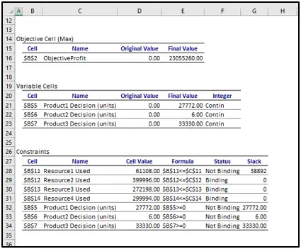
Solver found the best plan as producing 27,772 units of Product1, 6 units of Product2, and 33,330 units of Product3. This gives a maximum profit of $23,055,260. The solution uses Resources 2, 3, and 4 fully, while Resource1 still has spare capacity. This means the bottleneck resources are 2, 3, and 4 (Van et al. 2021). The solution satisfies all constraints, and no violations occur. The Answer Report confirms Solver’s output and shows which constraints are binding. This becomes the baseline scenario.
1f: Adding Product4
(Source: Self-Created in MS Excel)

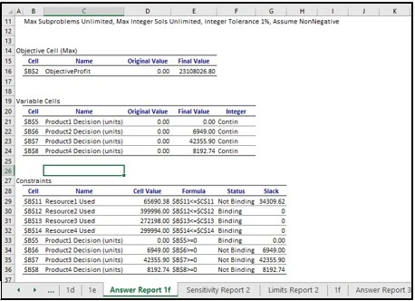
When Product4 was added, Solver produced a new plan. The company should make 6,949 units of Product2, 42,356 units of Product3, and 8,193 units of Product4, while Product1 is not produced. This gives a higher profit of $23,108,026.80, which is more than the base solution. This means adding Product4 is a good idea. Product4 contributes positively, and Solver shifts resources to balance production. Resources 2, 3, and 4 remain fully used, showing they are still bottlenecks.
1g: Profit Changes
(Source: Self-Created in MS Excel)
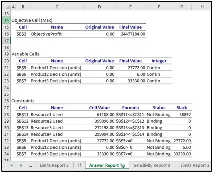
When Product1’s profit increased, Product2’s profit slightly decreased, and Product3’s profit increased by one, the Solver solution stayed the same. The company should still produce 27,772 units of Product1, 6 units of Product2, and 33,330 units of Product3 (Lubin et al. 2023). Profit, however, rose to $24,477,184 because of the profit changes.
1h: Integer Constraints
(Source: Self-Created in MS Excel)
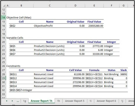
When the model required integer values for products, Solver gave the same solution as before. The company should produce 27,772 units of Product1, 6 units of Product2, and 33,330 units of Product3. Profit remains $23,055,260, showing that rounding did not affect results. All constraints are satisfied, with Resources 2, 3, and 4 still fully used, and Resource1 partly unused. This confirms that the integer restriction does not change the optimal outcome in this case.
1i: Startup Costs
When fixed startup costs were added, Solver still chose to produce 27,772 units of Product1, 6 units of Product2, and 33,330 units of Product3. The total profit remained $23,055,260 because all three products were still worth producing even after paying setup charges (Kashefi & Mukerji, 2023). The binary variables for each product were set to 1, showing all products were activated. Resource2, Resource3, and Resource4 stayed fully used, while Resource1 had spare capacity. This confirms startup costs did not change the mix.
1j: Linking Constraint
(Source: Self-Created in MS Excel)
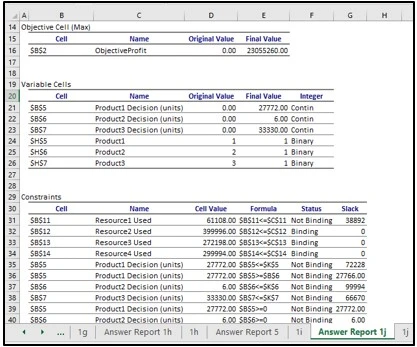
The model added a rule that if Product2 was made, Product1 should be at least as large as Product2. Solver’s solution remained unchanged at 27,772 units of Product1, 6 units of Product2, and 33,330 units of Product3 (An, Mikhaylov & Jung, 2021). The linking constraint was satisfied because Product1 is much larger than Product2. The total profit stayed at $23,055,260. Resources 2, 3, and 4 continued to bind, while Resource1 was not fully used. This shows the new rule did not affect the optimal plan.
1k: Minimum Percentage Rule
(Source: Self-Created in MS Excel)
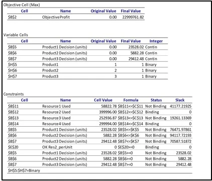
The new condition required Product2 to be at least 10% of the total production. Solver adjusted the plan by increasing Product2 to 5,882 units, reducing Product1 to 23,528 units and Product3 to 29,412 units (Qiu, Sun & Yang, 2022). The profit dropped slightly to $22,999,761.82, showing the new condition forced a less efficient mix. Resource2 and Resource4 stayed fully used, but Resource3 was no longer binding. This confirms that meeting the minimum percentage for Product2 caused a lower but still feasible profit.
1l: Batch Production Rule
(Source: Self-Created in MS Excel)
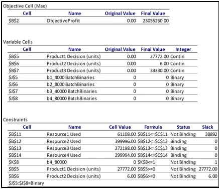
When the batch production rule for Product3 was applied, Solver chose the same plan as earlier. The company should make 27,772 units of Product1, 6 units of Product2, and 33,330 units of Product3. None of the batch binary variables were activated, meaning Solver treated Product3’s production level as already matching a feasible outcome (Xavier, Qiu & Ahmed, 2021). The maximum profit stayed at $23,055,260. Resources 2, 3, and 4 continued to bind, while Resource1 still had spare capacity.
1m: Startup and 27,000 Limit
(Source: Self-Created in MS Excel)
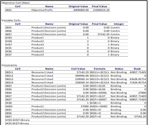
With new startup costs and the condition that no more than one product could exceed 27,000 units, Solver gave a different result. Product3 became the only product produced, at about 57,142 units. Product1 and Product2 were not made (Xiang & Connolly, 2022). The profit dropped to $21,856,914.29 after paying the startup cost for Product3. This shows that strict rules reduce flexibility and can lower total profit. Resource2 was still binding, but Resource3 and Resource4 were no longer fully used.
Question 2
2a Base Model Formulation and Solution
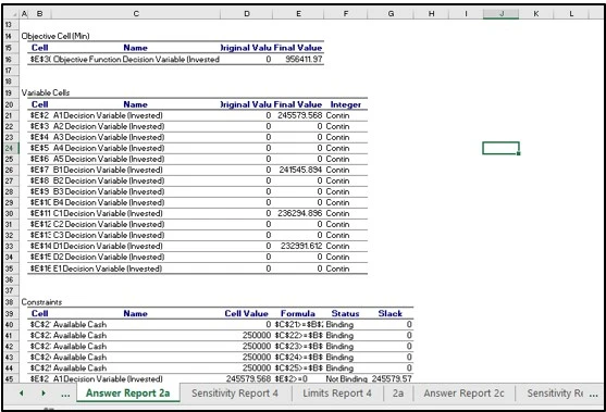
In Question 2a, the Solver found the lowest total investment needed was about $956,412. The fund achieves the cafeteria payments by spreading money across four key investments: A1, B1, C1, and D1. This combination ensures exactly $250,000 is available in months 2 to 5. All other investments remain unused since they are not cost-efficient.
2b Excel Solver Implementation
(Source: Self-Created in MS Excel)
In Question 2b, the Solver results are shown in Excel with the same objective of minimising total investment. The solution again highlights A1, B1, C1, and D1 as the main choices, as these provide the exact timing of cash flows required. The output clearly demonstrates that the Solver meets all constraints while keeping investment as low as possible.
2c Additional Constraint on D1 and C1
(Source: Self-Created in MS Excel)
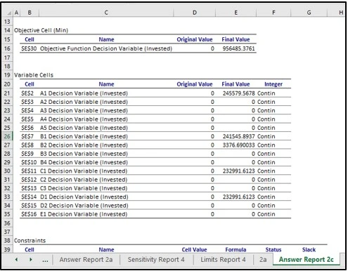
In Question 2c, an extra rule was added: investment D1 must be at least as large as C1. Solver adjusted by investing about $232,992 in both D1 and C1, and added a small amount in B2 to balance the payments. The new minimum investment rose slightly to $956,485, which is only a little higher than in 2a. This shows that adding more restrictions reduces flexibility and increases total cost, but the Solver still finds a workable plan.
2d Limiting to Four Investments
(Source: Self-Created in MS Excel)
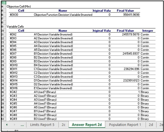
In Question 2d, the Solver added a restriction that only four investments could be used. The optimal plan still selected A1, B1, C1, and D1, which were already the best choices earlier. The total required investment stayed the same at about $956,412, and all cafeteria payments were met on time. This shows that the previous solution already relied on only four investments, so the new constraint did not change the result but confirmed the efficiency of the strategy.
2e Adding Investment Penalty Cost
(Source: Self-Created in MS Excel)
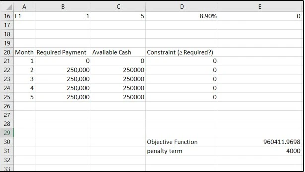
In Question 2e, a penalty of $1,000 per investment was added to the objective function. Since four investments were used, the penalty increased the cost by $4,000, raising the total to about $960,412. The Solver again chose A1, B1, C1, and D1 to cover the payments, because these were still the most efficient choices. This result shows that adding a fixed cost per investment increases overall expenses but does not change the chosen investments when they are already optimal.
Reference List
Journals
- An, J., Mikhaylov, A., & Jung, S. U. (2021). A linear programming approach for robust network revenue management in the airline industry. Journal of Air Transport Management, 91, 101979, retrieved from, https://www.academia.edu/download/97875484/1_s2.0_S0969699720305615_main.pdf [Retrieved on 1.9.2025]
- Cohen, M. B., Lee, Y. T., & Song, Z. (2021). Solving linear programs in the current matrix multiplication time. Journal of the ACM (JACM), 68(1), 1-39, retrieved from, https://dl.acm.org/doi/pdf/10.1145/3424305 [Retrieved on 1.9.2025]
- Kashefi, A., & Mukerji, T. (2023). ChatGPT for programming numerical methods. Journal of Machine Learning for Modeling and Computing, 4(2), retrieved from, https://arxiv.org/pdf/2303.12093 [Retrieved on 1.9.2025]
- Li, C., Conejo, A. J., Liu, P., Omell, B. P., Siirola, J. D., & Grossmann, I. E. (2022). Mixed-integer linear programming models and algorithms for generation and transmission expansion planning of power systems. European Journal of Operational Research, 297(3), 1071-1082, retrieved from, https://www.sciencedirect.com/science/article/am/pii/S0377221721005397 [Retrieved on 1.9.2025]
- Lubin, M., Dowson, O., Garcia, J. D., Huchette, J., Legat, B., & Vielma, J. P. (2023). JuMP 1.0: Recent improvements to a modeling language for mathematical optimization. Mathematical Programming Computation, 15(3), 581-589, retrieved from, https://arxiv.org/pdf/2206.03866 [Retrieved on 1.9.2025]
- Qiu, R., Sun, Z., & Yang, Y. (2022). Dimes: A differentiable meta solver for combinatorial optimization problems. Advances in Neural Information Processing Systems, 35, 25531-25546, retrieved from, https://proceedings.neurips.cc/paper_files/paper/2022/file/a3a7387e49f4de290c23beea2dfcdc75-Paper-Conference.pdf [Retrieved on 1.9.2025]
- Turner, M., Koch, T., Serrano, F., & Winkler, M. (2023). Adaptive cut selection in mixed-integer linear programming. Open Journal of Mathematical Optimization, 4, 1-28, retrieved from, https://www.numdam.org/item/10.5802/ojmo.25.pdf [Retrieved on 1.9.2025]
- Van Den Brand, J., Lee, Y. T., Liu, Y. P., Saranurak, T., Sidford, A., Song, Z., & Wang, D. (2021, June). Minimum cost flows, mdps, and ℓ1-regression in nearly linear time for dense instances. In Proceedings of the 53rd Annual ACM SIGACT Symposium on Theory of Computing (pp. 859-869), retrieved from, https://dl.acm.org/doi/pdf/10.1145/3406325.3451108 [Retrieved on 1.9.2025]
- Xavier, Á. S., Qiu, F., & Ahmed, S. (2021). Learning to solve large-scale security-constrained unit commitment problems. INFORMS Journal on Computing, 33(2), 739-756, retrieved from, https://arxiv.org/pdf/1902.01697 [Retrieved on 1.9.2025]
- Xiang, H., & Connolly, J. A. (2022). GeoPS: An interactive visual computing tool for thermodynamic modelling of phase equilibria. Journal of Metamorphic Geology, 40(2), 243-255, retrieved from, https://perplex.ethz.ch/papers/Xiang_JMG_2021.pdf [Retrieved on 1.9.2025]