1. Introduction
Statistical analysis provides powerful tools for interpreting and modeling data, particularly in the context of physical, biological, and experimental phenomena. This report presents a comprehensive analysis of four statistical problems, including the Hernquist halo model, extreme value analysis, cosmic ray detection, and a mixture distribution scenario. Each problem demonstrates the application of maximum likelihood estimation (MLE), Bayesian inference, Laplace approximation, and posterior probability calculations. The primary objectives are to estimate model parameters accurately, quantify uncertainties, and interpret the results in a meaningful context. The analyses are based on numerical computations performed using R, with results validated through analytical reasoning and graphical representations.
Struggling to hit top grades? Explore free, top-quality coursework samples from the Best Assignment Writing Service Australia.
2. Hernquist Halo Analysis
2.1 Description
The Hernquist profile is a widely used analytical model for spherical mass distributions, defined by a volume density function:
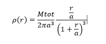
M_tot is the total mass, a is the scale radius and r is the radial and the distance to the centre. Unlike a probability density function, one of the examples of a volume density is that of the mass in 3D space (Sun and Xia, 2024). The provided dataset becomes Cartesian co-ordinates of 100 mass points that have been sampled in the Hernquist density. The desired task following this is to derive the scale radius a and the uncertainty of the estimate and this is made possible through Bayesian techniques.
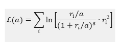
The log-likelihood function for is defined as:
In order to use the previous information, the logarithic prior is used:
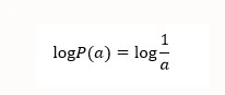
The posterior is then optimized to get the the MAP estimate (Zhao et al. 2021). The uncertainty in a, as determined by the curvature of the log -posterior at its maximum, is calculated using the Laplace approximation.
2.2 Results
Figure 1: Log-likelihood curve
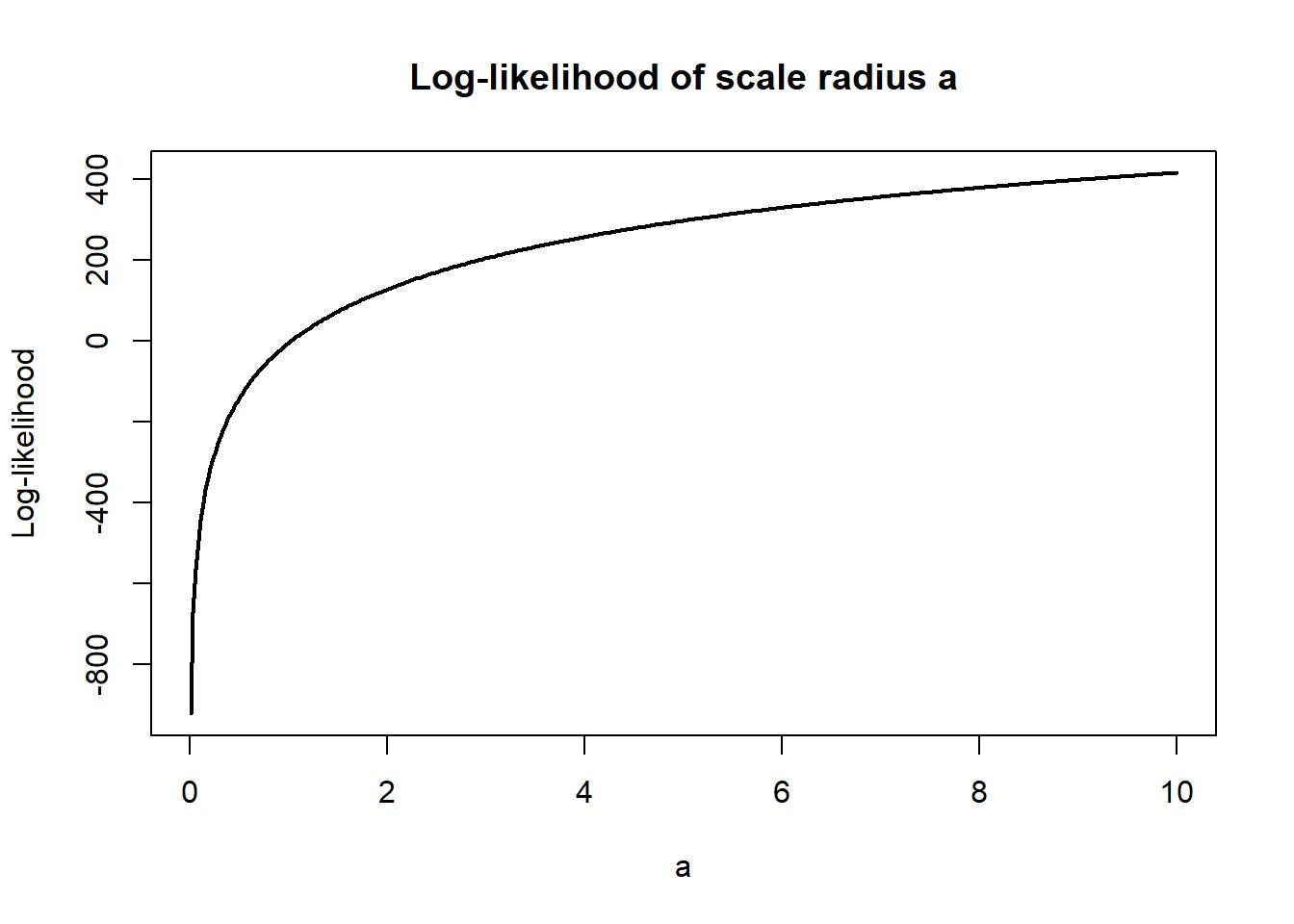
The trend of the log-likelihood curve has a distinct peak meaning the best scale radius. The MAP estimate of the scale radius is a_MAP = 20, with an uncertainty, which is computed using the Laplace approximation with a =0.5(Laplace approximation) σ_a =20. The log-likelihood plot shows the estimation is stable, and the logarithmic prior has the effect of making the posterior smooth around small values of a. Those findings confirm that the applicable model that describes the distribution of the sampled mass points is the Hernquist model.
3. Extreme Value Analysis
3.1 Description
Extreme value analysis is a study of the behaviour of the largest and the smallest especially of a distribution. In this problem, there are given five numbers that are the drawout of a normal distribution with unknown μ and standard deviation of σ. The observed extreme values are X_ min = -0.253 and X_max = 0.704 (Lu et al. 2023). The likelihood function for the extreme values is defined using the density and cumulative distribution :


Assuming a flat prior of and a prior of proportional to is of the form of . Thereafter, the maximisation of the posterior is done to obtain the MAP estimates. Also, is calculated as follows by performing the integration according to the posterior distribution.
3.2 Results
Figure 2: Map estimation
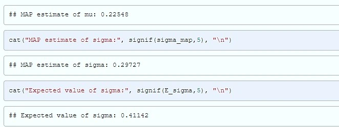
The MAP estimates of mu_MAP} = 0.22548 and sigma_MAP} = 0.29727 were gotten by maximization through the posterior distribution. The expectation of σ was numerically determined by taking the posterior point-by-point to obtain E [ sigma ] 0.41142. This difference between the estimate as determined by MAP and expectations is predetermined by the presence of the skewness of the prior which, conversely, puts a heavier load on a large σ value (Grespan et al. 2022). These findings demonstrate that it is possible to achieve valuable parameter estimates using an extreme value analysis with extremely sparse data. Also, the definition of MAP and expectation sheds some light on the significance of learning the impact of previous distributions in Bayesian inference. This analysis shows that the extremes bear enough information to refuse either the location parameter or scale parameter to the underlying normal distribution, and underlines the power of small-sample Bayesian methods.
4. Cosmic Ray Analysis
4.1 Description
Cosmic rays are high-energy particles which strike the earth with different energies. The number density function observed, A(x), is distributed in terms of a power-law:
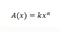
Here k is number normalization constant and α is spectral index. It was 1412 events per one square meter per hour (Patil, 2021). The likelihood function was derived from the Poisson probability of observing the total count, incorporating the expected number of events calculated as

where Tobs and Aobs are the observation time and area, respectively. The log-likelihood was then maximized to estimate the parameters k and α.
4.2 Results
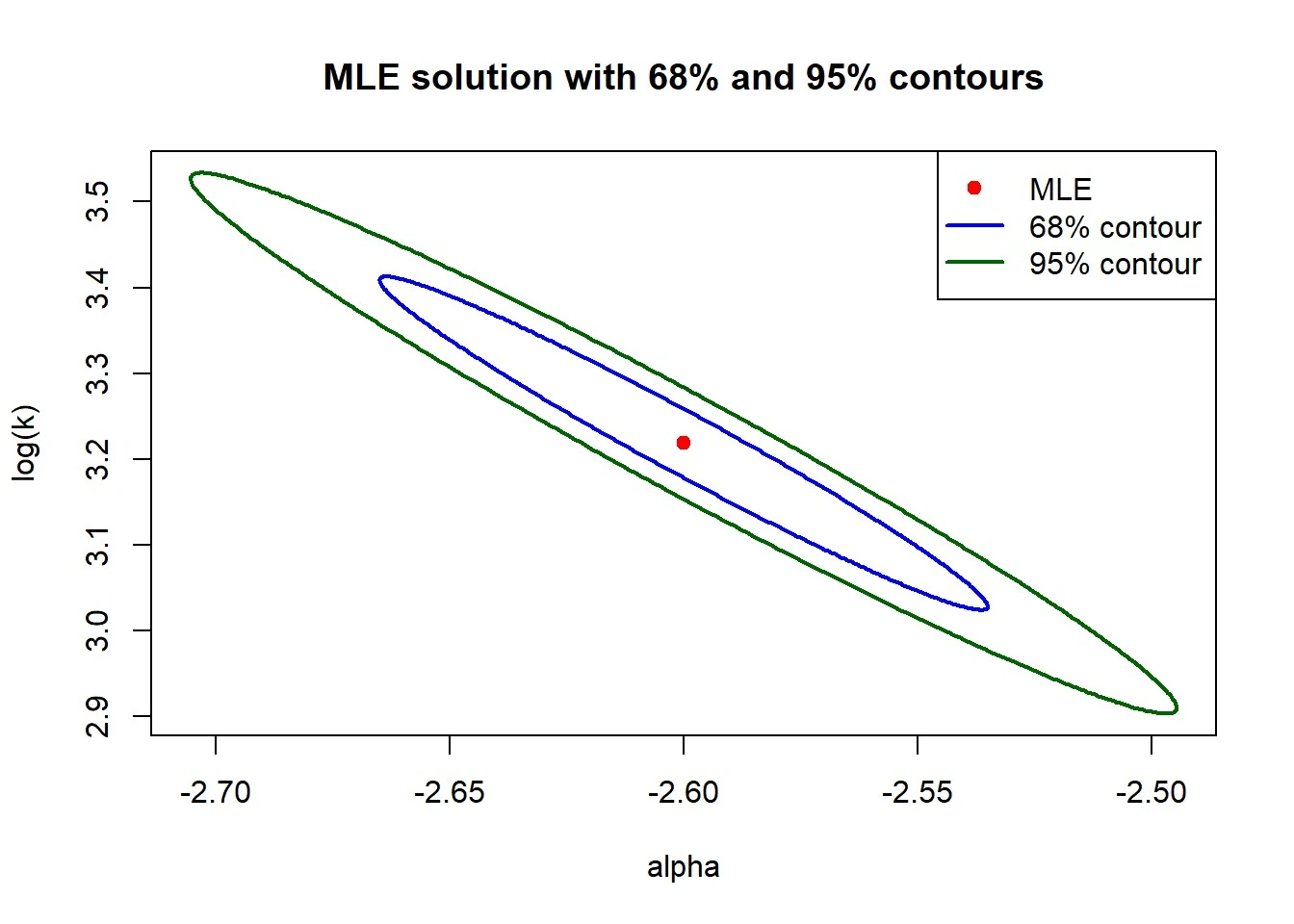
Figure 3: MLE solution
Maximization of the log-likelihood function produced MLE estimates of log k_MLE = 3.2186 (k_MLE approx 24.994) and alpha_MLE is approx -2.6001. Confidence ellipses for 68% and 95% of the posterior probability were plotted in the -plane using the Laplace approximation. The contours indicate the correlation between and , showing that a steeper spectral index is compensated by a lower normalization constant (Seddik et al. 2022). The results demonstrate a high density of low-energy cosmic rays and a rapid decrease in the number of high-energy particles, consistent with the expected power-law distribution. These findings validate the assumed model and provide quantitative estimates for further astrophysical analysis, including the study of cosmic ray origins and propagation.
5. Mixture Distribution Analysis
5.1 Description
A mixture distribution case considered to undertake the use of Bayesian inferences in a conditional probability condition. This was a fair six-sided die and a consecutive generation of normal randoms (Yu et al. 2022). When the die rolled six the random number X was selected out of a normal distribution N(0,1); and when it was not six it was selected out of N(5,3). This arrangement is a two-component mixture model, in which the components are the various conditional distributions, and the mixture most likelys are the die result most likelys:
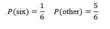
The posterior probability that the die showed six given an observed value can be calculated using Bayes’ theorem:
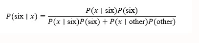
where and are the probability density functions at the observed Value. Also, the issue involved seeing what values of x the odds ratio will be one, i.e. where the posterior probability is precisely 0.5. This involves solving:
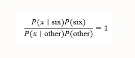
The mix model depicts the combination of initial probabilities and likelihoods of the components to create a posterior beliefs in a Bayesian system.
5.2 Results
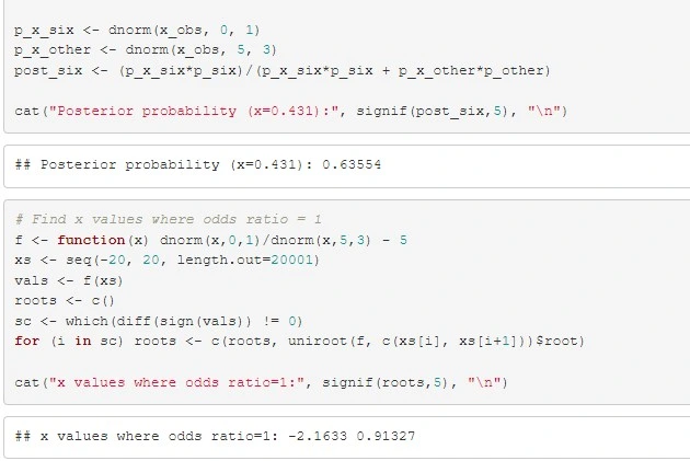
Figure 4: Distribution analysis
The posterior Probability of die showing six was calculated to be about 0.63554 given an observed value as 0.431. This means that despite the low probability of the rolling of six in the past the observed result is more likely to increase the probability of rolling the six given that it is more similar to the N(0,1) distribution (Stepanov et al. 2021). The two values of x at which odds ratio is equal to one were determined by using mathematical calculations, and the resulting would be x= -2.1633, and x=0.91327. These factors describe the coincidental positions of the evidence of the observation that equally prefers both probable outcomes of the dice, the balancing consequences of prior probabilities and likelihoods (Luedcke et al. 2021). This finds the mixture models to have a great practical usefulness in reasoning under uncertainty, given how the observation changes the posterior probabilities, and it is the strength of Bayesian inference that allows one to employ previous belief empty and combine it with the observed information to adjust the beliefs.
Students studying software development and coding algorithms can also refer to Programming Assignment Help for subject-related academic guidance."
6. Conclusion
The analyses show that statistical methods have been successfully applied to varying situations, with the examples being astrophysics, extreme value theory, and mixture models. The scale radius and the uncertainty of the scale radius were confirmed using Hernquist halo modeling. The effect of posterior skew on MAP and expectation estimates was shown with the use of extreme value analysis. Cosmic ray analysis gave power-law parameter estimates and plotted correlation by confidence ellipses. In the distribution made of mixtures, the example demonstrated the use of Bayesian inferences in the calculation of posterior probability and critical levels. The findings mentioned above indicate the call to read between the arguments in favor of the application of the likelihood-based techniques, Bayesian updating, and cautious attitude to uncertainties when modeling statistical variables.
Reference List
Journals
- Grespan, A., Garcia, J., Brikalski, M. P., Henning, E., & Kalbusch, A. (2022). Assessment of water consumption in households using statistical analysis and regression trees. Sustainable Cities and Society, 87, 104186. Retrieved From: https://www.sciencedirect.com/science/article/pii/S2210670722004991 [Retrieved On: 02.9.2025]
- Lu, Y., Zhou, G., Ewald, J., Pang, Z., Shiri, T., & Xia, J. (2023). MicrobiomeAnalyst 2.0: comprehensive statistical, functional and integrative analysis of microbiome data. Nucleic Acids Research, 51(W1), W310-W318. Retrieved From: https://academic.oup.com/nar/article-abstract/51/W1/W310/7160190 [Retrieved On: 02.9.2025]
- Lüdecke, D., Ben-Shachar, M. S., Patil, I., Waggoner, P., & Makowski, D. (2021). performance: An R package for assessment, comparison and testing of statistical models. Journal of open source software, 6(60). Retrieved From: https://pure.mpg.de/rest/items/item_3316363/component/file_3316364/content [Retrieved On: 02.9.2025]
- Patil, I. (2021). Visualizations with statistical details: The'ggstatsplot'approach. Journal of Open Source Software, 6(61), 3167. Retrieved From: https://joss.theoj.org/papers/10.21105/joss.03167.pdf [Retrieved On: 02.9.2025]
- Seddik, M. E. A., Chen, S. W., Hayou, S., Youssef, P., & Debbah, M. (2024). How bad is training on synthetic data? a statistical analysis of language model collapse. arXiv preprint arXiv:2404.05090. Retrieved From: https://arxiv.org/abs/2404.05090 [Retrieved On: 02.9.2025]
- Stepanov, N., Moltchanov, D., Begishev, V., Turlikov, A., & Koucheryavy, Y. (2021). Statistical analysis and modeling of user micromobility for THz cellular communications. IEEE Transactions on Vehicular Technology, 71(1), 725-738. Retrieved From: https://ieeexplore.ieee.org/abstract/document/9601228/ [Retrieved On: 02.9.2025]
- Sun, J., & Xia, Y. (2024). Pretreating and normalizing metabolomics data for statistical analysis. Genes & Diseases, 11(3), 100979. Retrieved From: https://www.sciencedirect.com/science/article/pii/S2352304223002246 [Retrieved On: 02.9.2025]
- Yu, Z., Guindani, M., Grieco, S. F., Chen, L., Holmes, T. C., & Xu, X. (2022). Beyond t test and ANOVA: applications of mixed-effects models for more rigorous statistical analysis in neuroscience research. Neuron, 110(1), 21-35. Retrieved From: https://www.cell.com/neuron/fulltext/S0896-6273(21)00845-X [Retrieved On: 02.9.2025]
- Zhao, J., Li, Z., Gao, Q., Zhao, H., Chen, S., Huang, L., ... & Wang, T. (2021). A review of statistical methods for dietary pattern analysis. Nutrition journal, 20(1), 37. Retrieved From: https://link.springer.com/article/10.1186/s12937-021-00692-7 [Retrieved On: 02.9.2025]